CPSC 406: In class activity 1 (Due date: Feb 26, 6pm)¶

In homework 2, you used Convex.jl to minimize multi-objective problems. Ready-built solvers are great tools for prototyping, because it helps limit bugs to modeling errors. However, often there is a tradeoff, whether in scalability, or in generality. In this homework, you will program your own optimization methods on several machine learning problems.

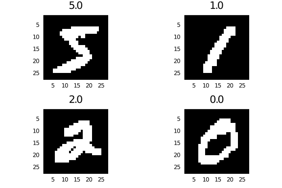
Retrieving data. Download mnist.mat. This dataset contains 28 x 28 black and white images of handwritten digits, 0,...,9. Install package MAT to open and read the dataset.

using MAT, Plots, Images, LinearAlgebra, ImageView, Colors, Statistics
# open file
file = matopen("mnist.mat")
trainX = float64.(read(file, "trainX"))
trainY = float64.(read(file, "trainY"))
testX = float64.(read(file, "testX"))
testY = float64.(read(file, "testY"));

The actual picture itself has been vectorized. To view image $i$ (where, for the trainig set, $i = 1,...,60000$ ) type the following commands

i = 1
img = reshape(trainX[i,:], 28, 28)';
img = heatmap(Gray.(img))
plot(img, title = "$(trainY[i])", axis = false)

You should get one of the 4 images show below.

Preprocessing In this homework you will implement several binary classification models in order to disambiguate 4 from 9. In order to do so, we need a matrix $A\in \R^{m\times n}$ where $m = \red{?}$ is the number of training samples, and $n = 28\times 28 = 784$ is the feature length. Additionally, we need a vector $b\in \R^m$ where $b_i = +1$ if the $i$ th sample is a 4, and $-1$ if it is a 9. As in many data science projects, the first step is in processing the data in order to find these constants.
1. First, filter out all the datapoints in the test and train set corresponding to any sample that is not a 4 or 9. With the train data, this can be done using
```
# pull out 4s and 9s from train set
idx4 = trainY .== 4 
idx9 = trainY .== 9
idx = idx4 + idx9
idx = findall(x->x == 1, idx[1,:])

A = trainX[idx,:]
b = trainY[idx]
```
  Do something similar to generate Atest and btest.
2. Now, transform $b$ so that instead of taking labels 4 and 9, it takes labels +1 and -1.
3. De-biasing and normalizing Two tricks that often make models work a lot better is removing the bias and making the variance as close to 0 as possible. To remove the bias, perform
```
Amean = mean(A, dims=1);
A = A - ones(m,1)*Amean;
```
  To remove the variance, perform
```
Astd = std(A, dims=1);
A = A ./ (ones(m,1)*max.(Astd,1));
```
  The extra normalization of the denominator is to avoid dividing by 0. Note that order matters; we cannot remove the variance before removing the mean. (Why?) Note also we actually divide by the standard deviation of $X$ , which is the square root of the variance.
We now have our data matrix $A$ and label matrix $b$ corresponding to the training set. Now, we want

$x_{LS} = \argmin_x \|Ax-b\|_2^2$
1. Solve this using a direct method (e.g. $A \backslash b$ ). Evaluate the loss of the model
  
  $\text{loss}(x_{LS}) = \|Ax-b\|_2^2.$
2. Discuss how to now construct a classifier, e.g. some function $C_x(a)$ that takes some feature vector $a\in \R^m$ and returns $+1$ if the image is a 4, and $-1$ otherwise. Evaluate the training misclassification rate
  
  $\texttt{train misclass rate}(x_{LS}) = \frac{1}{m}\sum_{i=1}^m I(C_{x_{LS}}(A_i), b_i)$
  
  where $I(x,y) = 1$ if $x\neq y$ and $I(x,y) = 0$ if $x = y$ .
3. Both the loss and training error are good ways of evaluating how well we did in both fitting the model and solving the optimization problem. However, it can only tell us about data we already observed. We don't know what will happen with data we haven't yet seen. To do this, we need to evaluate the testing error.
  
  However, before using the testing data, we must first preprocess it in exactly the same way we preprocessed the training data. That means using the same vector for both the mean and the standard deviation, computed from the trainig data alone.
  
  To preprocess the training data, run
```
Atest = Atest - ones(mtest,1)*Amean;
Atest = Atest./(ones(mtest,1).*max.(Astd,1));
```
  without recomputing Amean or Astd. Discuss briefly why not recomputing these constants is so important.
Linear regression models are a great "first pass" algorithm to classify data, because they are so easy to implement, and can be used to double check if the data preprocessing was done correctly. However, there are many reasons why they may not be the best classification tool. In the second half, we will investigate a slightly more sophisticated model, more suited for classification.
Logistic regression Rather than fitting data linearly to labels +1 and -1, in logistic regression, we are fitting a likelihood to 0 or 1.

Specifically, for a data vector $a\in \R^n$ and label $b\in \{0,1\}$ , we define the probability that label $b$ is associated with data vector $a$ as

$\text{Likelihood} = \pr(\text{data}|\text{obs}) = \pr(b|a,x) = \begin{cases} \sigma(a_i^Tx) & \text{ if } b = 1,\\ 1-\sigma(a_i^Tx) & \text{ if } b = 0 \end{cases}$

where

$\sigma(s) = \frac{1}{1+e^{-s}}$

is the sigmoid function (plotted below.)

This function can be interpreted as a "soft switching" function; the input $s$ can be viewed as a "confidence level" of the prediction, and is large and positive if you believe $b = 1$ , and large and negative if you believe $b = 0$ . When the prediction is not confident, then the output is close to 0. The idea here is that by fitting this model, we don't add numerical artifacts by being "too confident"--e.g. no very large numbers as a result of good data.

Now assume that for our training data $\{a_1,...,a_m\}$ and labels $\{b_1,...,b_m\}$ are i.i.d. Then the likelihood of observing this entire training set is

$\text{Likelihood} = \prod_{i=1}^m\pr(b_i|a_i,x) = \prod_{i=1}^m \sigma(a_i^Tx)^{b_i} (1-\sigma(a_i^Tx))^{1-b_i}$

where the last step incodes the case switching.

Our goal is to maximize this likelihood. However, this function is not convex, and is rather complicated; computing the gradient or Hessian is not trivial. Therefore, we maximize the log likelihood, solving instead

$\maximize_{x} \quad f(x) := \log\left(\prod_{i=1}^m \sigma(a_i^Tx)^{b_i} (1-\sigma(a_i^Tx))^{1-b_i}\right) .$

The loss function is the negative log likelihood.
1. Conceptual questions.
  1. Explain why it is equivalent to maximize the log likelihood and likelihood.
  2. Simplify the loss function, and derive the gradient and Hessian. Is the function convex, concave, or neither?
2. Coding questions
  1. In logistic regression, we are dealing with 0,1 labels rather than -1,1 labels. To fix this, take the $b$ vector and readjust: for example, b = (b+1)/2.
  2. Using an initial value $x^{(0)} = 0$ , code up gradient descent to minimize this new loss function. Run for 1000 iterations with fixed step size $1/m$ ( m = total number of training samples.) Plot the model loss as a function of iteration, and report the final train and test misclassification rate.
    
    (If you worry that $\log(\sigma(a_i^Tx))=-\infty$ or $\log(1-\sigma(a_i^Tx))=-\infty$ because the sigmoid function returns 0 or 1, you may replace $\sigma(a_i^Tx)$ with $\max(\min(\sigma(a^T_i x),\epsilon),\epsilon)$ where $\epsilon$ is some small number.)
  3. Using an initial value $x^{(0)} = 0$ , code up gradient descent to minimize this new loss function. Run for 1000 iterations with a backtracking line search with $s = 1$ , $\alpha = \beta = 0.5$ . Plot the model loss as a function of iteration, and report the final train and test misclassification rate.
  4. Compare in 1-2 sentences gradient descent with line search vs constant step size. Which is better?
  5. Compare in 1-2 sentences the linear and logistic model. Which is better? Is it better by much? Was the gain worth it?
Debugging Pick three images that fit the leasts squares model the worst, and plot them. Do the same with the logistic model.