Least Squares

In this lecture, we will cover least squares for data fitting, linear systems, properties of least squares and QR factorization.

Least squares for data fitting

Consider the problem of fitting a line to observations $y_i$ gven input $z_i$ for $i = 1,\dots, n$.

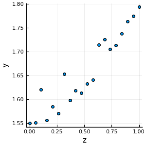
In the figure above, the data points seem to follow a linear trend. One way to find the parameters $c,s \in \R$ of the linear model $f(z) = s\cdot z + c$ that coresponds to a line of best fit is to minimize the following squared distance subject to a linear constraint:

$$\begin{align*} \min_{s,\,c,\,\hat{y}_i \in \R} &\sum_{i=1}^n (y_i - \hat{y}_i)^2\\ \text{subject to } &s\cdot z_i+c = \hat{y}_i \end{align*}$$

The above minimization program can be reformulated as a linear least squares problem:

$$\min_{\vx} \|\mA \vx - \vb\|_2^2 = \sum_{i=1}^n(\va_{i}^\intercal\vx-b_i)^2,$$

where

$$\mA = \begin{bmatrix}z_1 & 1\\ z_2 & 1\\ \vdots&\vdots\\z_n & 1\end{bmatrix}, \ \vb = \begin{bmatrix}y_1\\y_2\\\vdots \\y_n\end{bmatrix}, \text{ and } \vx = \begin{bmatrix}s\\c\end{bmatrix}.$$

Let

$$\begin{equation}\label{least_squares_problem} \func{f}(\vx):=\frac{1}{2}\|\mA\vx-\vb\|_2^2 = \frac{1}{2}\sum_{i=1}^n(\va_{i}^\intercal\vx-b_i)^2. \end{equation}$$

The gradient and hessian of $\func{f}(\vx)$ are:

$$\nabla\func{f}(\vx) = \mA^\intercal(\mA\vx-\vb), \text{ and } \nabla^2\func{f}(\vx) = \mA^\intercal\mA,$$

respectively. The Hessian is positive semidefinite for every $\vx$ (and is positive definite if $\mA$ has full row rank). This implies that the function $\func{f}(\vx)$ is convex. Additionally, $\vx = \vx^{*}$ is a critical point if

$$\begin{equation}\label{least_square_normal_eqn} \mA^\intercal(\mA\vx^*-b) = \vzero. \end{equation}$$

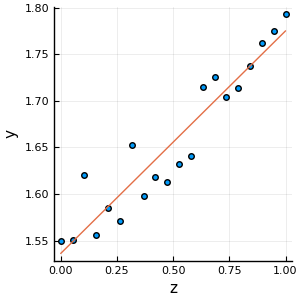
Since $\func{f}(\vx)$ is convex, $\vx^{*}$ is a global minimizer. Equation \eqref{least_square_normal_eqn} is called the normal equations of the least squares problem \eqref{least_squares_problem}. Solving the normal equations, we get the following line of best fit.

Linear systems

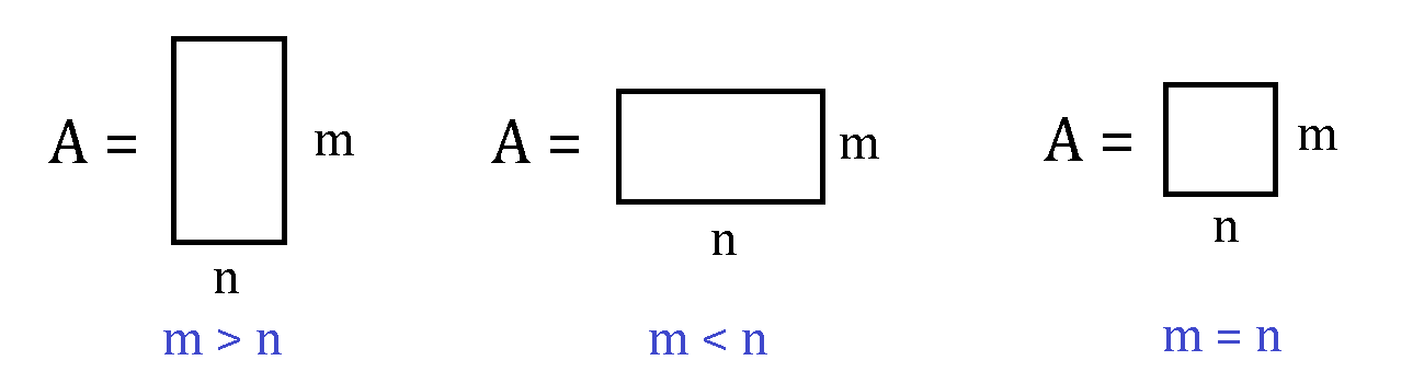
Consider the problem of solving a linear system of equations. For $\mA \in \R^{m\times n}$ and $\vb\in\R^{m}$, the linear system of equations $\mA\vx = \vb$ is:

1. overdetermined if $m>n$,
2. underdetermined if $m< n$, or
3. square if $m = n$.

A linear system can have exactly one solution, many solutions, or no solutions:

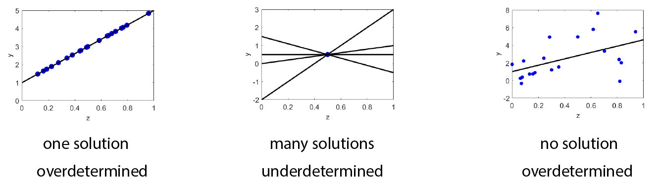
In general, a linear system $\mA\vx=\vb$ has a solution if $\vb \in \text{range} (\mA)$.

Properties of linear least squares

Recall that the minimizer $\vx^*$ to the linear least squares poblem satisfies the normal equations:

$$\mA^\intercal \mA \vx^* = \mA^\intercal\vb$$

with the residual

$$\vr^* = \mA\vx^* -\vb,$$

satisfying $\mA^\intercal\vr^* = \vzero.$ Here, $\mA \in \R^{m\times n}$. The minimzer of the linear least squares problem is unique if $\mA^\intercal\mA$ is invertible. However, the vector in the range of $\mA$ closest to $\vb$ is unique, i.e. $\vb^* = \mA\vx*$ is unique. Recall that range space of $\mA$ and the null space of $\mA^\intercal$ is:

$$\text{range}(\mA) = \set{R}(\mA) = \{\vy : \vy = \mA \vx \text{ for some } \vx \}\\ \text{null}(\mA^\intercal)= \set{N}(\mA^\intercal) = \{\vz: \mA^\intercal\vz = \vzero\}$$

By fundamental theorem of linear algebra, we have $$ \begin{equation}\label{least_squares_FTLA} \set{R}(\mA) \oplus \set{N}(\mA^\intercal) = \R^m. \end{equation} $$ Thus, for all $\vx \in \R^m$, we have

$$\vx = \vu + \vv, \quad \vu \in \set{R}(\mA), \quad \vv\in\set{N}(\mA^\intercal)$$

with $\vu$ and $\vv$ uniquely determined. This is illustrated in the figure below:

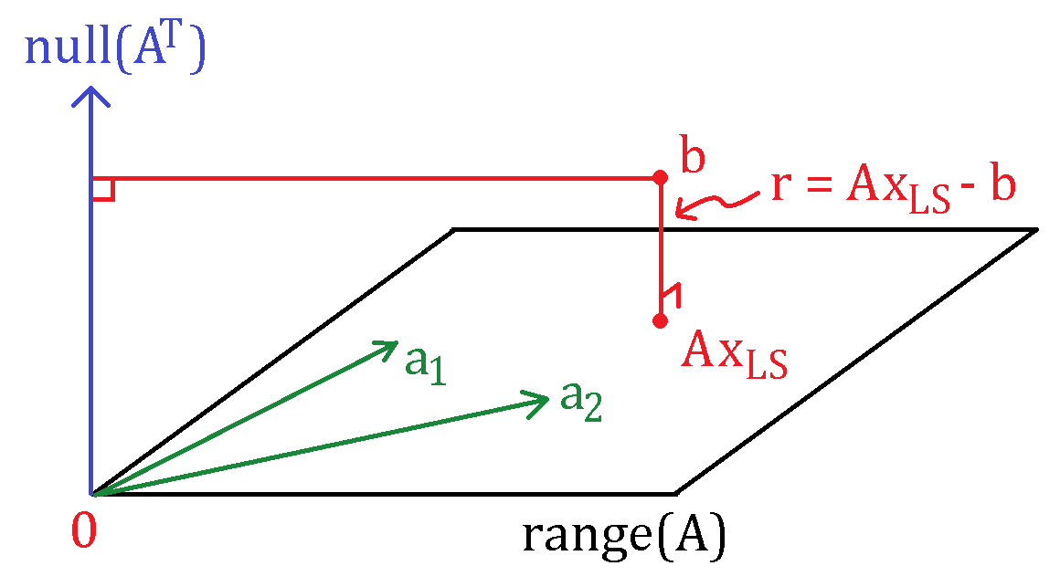
Here, $\vx_{LS}$ is the least squares solution, $\mA = \begin{bmatrix}\va_1&\va_2&\dots&\va_n\end{bmatrix}$, with $\va_i \in \R^m$ for all $i$. Comparing with \eqref{least_squares_FTLA}, we get

$$\vb = \mA\vx_{LS}+r \text{ with } \mA\vx_{LS} \in \set{R}(\mA) \text{ and } \vr \in \set{N}(\mA^\intercal)$$

$\exa{1}$ What is the least-squares solution $\vx^*$ for the problem

$$\min_{\vx} \frac{1}{2} \|\mA\vx - \vb\|_2^2,$$

where

$$\mA = \begin{bmatrix} 1 \\ \vdots \\ 1 \end{bmatrix} = \ve \in \R^m \quad \text{ and } \quad \vb = \begin{bmatrix} b_1 \\ \vdots \\ b_m \end{bmatrix}.$$

$\text{Solution:}$ First setup the normal equations:

$$\mA^\intercal\mA\vx = \begin{bmatrix}1&\dots&1\end{bmatrix} \begin{bmatrix} 1 \\ \vdots \\ 1 \end{bmatrix}\vx = m\vx \quad \text {and} \quad \mA^\intercal\vb = \begin{bmatrix}1&\dots&1\end{bmatrix} \begin{bmatrix} b_1 \\ \vdots \\ b_m \end{bmatrix} =\ve^\intercal\vb$$

Solving the normal equations, we get

$$\mA^\intercal\mA\vx^* = \mA^\intercal\vb \iff m\vx^* = \ve^\intercal\vb \iff \vx^* = \frac{1}{m}\ve^\intercal\vb$$

So, the least squares solution $\vx^*$ is the mean value of the elements in $\vb$.