Mathematical background

Vectors

Vectors are arrays of numbers ordered as a column. For example, a vector $\vx \in \R^n$ contain $n$ entries with $x_i$ as its $i$th entry:

$$\vx \in \R^n,\quad \vx = \begin{bmatrix} x_1\\ x_2\\ \vdots\\ x_n \end{bmatrix},\quad \vx = \begin{pmatrix}x_1, x_2,\dots,x_n\end{pmatrix}.$$

Some special vectors that are commonly used are the zero vector, ones vector, and the standard basis vectors. These are defined next:

1. Zero vector: A vector $\vx$ is the zero vector if all of its entries are zero. The zero vector is denoted by $\vzero$.
2. Ones vector: A vector $\vx$ is the ones vector if all of its entries are one. The ones vector is denoted by $\ve$.
3. $i$th standard basis vector: A vector $\vx \in \R^n$ is the $i$th standard basis vector if $x_j = \Big\{\begin{array}{cc}1 & i = j\\0 & \text{otherwise}\end{array}$. The $i$th standard basis vector is denoted by $\ve_i$. For example, in $\R^3$, the $2$nd standard basis vector is $\ve_2 = \begin{bmatrix}0\\1\\0\end{bmatrix}$.

A vector $\vx \in \R^n$ is equal to another vector $\vy \in \R^n$ if $x_i = y_i$ for all $i \in \{1,2,\dots,n\}$. Similarly, if all of the entries of a vector $\vx$ is equal to a scalar $c \in \R$, then we write $\vx = c$. These notions can be extended to inequalites in the following way:

1. A vector $\vx \in \R^n$ and a scalar $c \in \R$ satisfy $\vx \geq c$ if and only if $x_i \geq c$ for all $i \in \{1,2,\dots, n\}$.
2. A vector $\vx \in \R^n$ and a scalar $c \in \R$ satisfy $\vx > c$ if and only if $x_i > c$ for all $i \in \{1,2,\dots, n\}$.
3. Vectors $\vx, \vy \in \R^n$ satisfy $\vx \geq \vy$ if and only if $x_i \geq y_i$ for all $i \in \{1,2,\dots, n\}$.
4. Vectors $\vx, \vy \in \R^n$ satisfy $\vx \geq \vy$ if and only if $x_i \geq y_i$ for all $i \in \{1,2,\dots, n\}$.

Block vector is a concise representation of a vector obtained by stacking vectors. For example, if $\vx \in \R^m$, $\vy \in \R^n$, and $\vz \in \R^p$, then

$$\va = \begin{bmatrix} \vx \\ \dots \\ \vy \\ \dots \\ \vz\end{bmatrix}\in \R^{m+n+p}$$

is a block vector (also called stacked vector or conncatenated vector) obtained by stacking $\vx$, $\vy$, and $\vz$ vertically. This block vector $\va$ can also be written as $\begin{pmatrix}\vx,\vy,\vz \end{pmatrix}$. If the dimension of the vectors are equal (i.e. $m = n = p$), then these vector can be stacked horizontally as well. This will produce a matrix

$$\mB = \begin{bmatrix} \vx & \vy & \vz\end{bmatrix} \in \R^{n\times 3}$$

where $\vx,\vy$, and $\vz$ are the first, second, and third columns of $\mB$, respectively.

Matrices

A matrix is an array of numbers and is another way of collecting numbers. For example, a matrix $\mA \in \R^{m\times n}$ contain $n$ rows and $m$ columns with a total of $m\cdot n$ number of entries:

$$\mA \in \R^{m\times n}, \quad \mA = \begin{bmatrix}A_{1,1}& \dots & A_{1,n}\\\vdots&\ddots &\vdots\\A_{m,1}&\dots&A_{m,n}\end{bmatrix}.$$

The tranpose of this matrix $\mA$ is denoted by $\mA^\intercal\in\R^{n\times m}$ where

$$\mA^\intercal =\begin{bmatrix}A_{1,1}& \dots & A_{m,1}\\\vdots&\ddots &\vdots\\A_{1,n}&\dots&A_{m,n}\end{bmatrix}$$

A matrix $\mA$ is the zero matrix if all of its entrie are zero. The zero matrix is denoted by $\mzero$. For a matrix $\mA \in \R^{m\times n}$,

1. if $m>n$ then the matrix $\mA$ is a tall matrix,
2. if $m< n$ then the matrix $\mA$ is a wide matrix, and
3. if $m = n$ then the matrix $\mA$ is a square matrix.

Matrices $\mA$ and $\mB$ are equal if these matrices are of same size and every element is equal: $$ \mA = \mB \iff A_{ij} = B_{ij},\quad \forall i = 1,\dots,m, \quad j = 1,\dots,n. $$ If all of the entries of a matrix $\mA$ are a scalar $c \in \R$ then we write $\mA = c$. These notions are extended to inequalities in the following way:

1. $\mA \geq c$ if and only if $A_{ij} \geq c$ for all $i = 1,\dots,m$ and $j = 1,\dots,n.$
2. $\mA > c$ if and only if $A_{ij} > c$ for all $i = 1,\dots,m$ and $j = 1,\dots,n.$
3. $\mA \geq \mB$ if and only if these matrices are of same size and $A_{ij} \geq B_{ij}$ for all $i = 1,\dots,m$ and $j = 1,\dots,n.$
4. $\mA > \mB$ if and only if these matrices are of same size and $A_{ij} > B_{ij}$ for all $i = 1,\dots,m$ and $j = 1,\dots,n.$

Inner products

Inner product is a way to multiply two vectors and matrices to produce a scalar. For $\setV = \R^n\text{ or } \R^{m\times n}$, inner product is a map $\langle\cdot,\cdot\rangle:\setV\times \setV\rightarrow \R$ that satisfies the following properties for all $\vx, \vy, \vz \in \setV$ and $\alpha \in \R$:

1. Non-negativity: $\langle \vx,\vx\rangle \geq 0$ and $\langle \vx,\vx\rangle = 0$ if and only if $\vx = 0$.
2. Symmetry: $\langle \vx, \vy\rangle = \langle \vy,\vx\rangle$.
3. Linearity: $\langle\alpha \vx, \vy\rangle = \alpha \langle\vx,\vy\rangle$ and $\langle \vx+\vy,\vz\rangle = \langle\vx,\vz\rangle + \langle\vy,\vz\rangle$.

For $\setV = \R^n$, the Euclidean inner product between two vector $\vx, \vy\in\R^n$ is also denoted as $\vx^\intercal\vy$ and

$$\vx^\intercal\vy = x_1y_1+x_2+y_2+\dots+x_ny_n.$$

$\exa{1}$ Fix $i \in \{1,\dots,n\}$. The inner product of $i$th standard basis vector $\ve_i$ with an arbitary vector $\vx$ is the $i$th entry of $\vx$, i.e. $\ve_i^\intercal\vx = x_i$.

$\exa{2}$ The inner product of the vector of ones $\ve$ with an arbitary vector $\vx$ is in the sum of entres of $\vx$, i.e. $\ve^\intercal\vx = x_1+x_2+\dots+x_n$.

$\exa{3}$ The inner product on an arbitary vector $\vx$ with itself is the sum of squares of the entries of $\vx$, i.e. $\vx^\intercal\vx =x_1^2+x_2^2+\dots+x_n^2$.

$\exa{4}$ Let $\vp = (p_1,p_2,\dots,p_n)$ be a vector of prices and $\vq = (q_1,q_2,\dots,q_n)$ be the corresponding vector of quantities. The total cost is the inner product of $\vp$ and $\vq$, i.e. $\vp^\intercal\vq = \sum_{i = 1}^np_iq_i$.

$\exa{5}$ Let $\vw$ be a vector of assest allocations ($\ve^\intercal\vw = 1, \vw\geq 0$) and $\vp$ be the corresponding vector of asset prices. The total portfolio value is $\vw^\intercal\vp$.

For $\setV = \R^{m\times n}$, the trace inner product between two matrices $\mA, \mB \in \R^{m\times n}$ is also denoted as $\text{tr}(\mA^\intercal\mB)$ and

$$\trace{\mA^\intercal\mB} = \sum_{i=1}^m\sum_{j=1}^nA_{ij}B_{ij} =\vec{\mA}^\intercal\vec{\mB},$$

where for a square matrix $\mS \in \R^{n\times n}$, $\trace{\mS} =\sum_{i=1}^n S_{ii}$, and for a matrix $\mA$ with columns $\va_1,\va_2,\dots,\va_n \in \R^m$,

$$\vec{\mA} = \begin{bmatrix}\va_1 \\\va_2\\\vdots\\\va_n \end{bmatrix}.$$

Norms

Norms are a measure of distances of a vector from the origin. The most common norm is the "Euclidean norm", i.e. 2-norm:

$$\|\vx\|_2 = \sqrt{x_1^2+\dots+x_n^2}$$

This 2-norm is the norm induced by the Euclidean inner product on $\R^n$, where $\|\vx\|_2 = \sqrt{\vx^\intercal\vx}$. The 2-norm reults in the familiar pythagorean identity, i.e. for any vectors $\va, \vb,$ and $\vc$,

$$\|(\va,\vb,\vc)\|_2^2 = \|\va\|_2^2+\|\vb\|_2^2+\|\vc\|_2^2.$$

An important inequlity that relates the inner product of two arbitary vectors with the norms of those vectors induced by the inner product is the Cauchy-Schwartz inequality. In the case of $\R^n$, the Cauchy-Schwartz inequality states that for all $\vx, \vy \in \R^n$, we have

$$\vx^\intercal\vy \leq \|\vx\|_2\|\vy\|_2.$$

For $\R^n$, the Cauchy Schwartz inequality follows from the Cosine inequality, i.e. for any vectors $\vx, \vy$ with angle $\theta$ between $\vx$ and $\vy$, we have $\vx^\intercal \vy = \|\vx\|_2\|\vy\|_2\cos(\theta)$. So, the Cauchy-Schwartz inequality attains the equality if and only if the two vectors are co-linear.

The Cauchy-Schwartz inequality gives us another inequailty that norms, in general, satisfy. This inequailty is the triangle inequality and states that

$$\begin{equation}\label{background:triangle} \text{for any vectors } \vx, \vy \in \R^n,\ \|\vx+\vy\|_2\leq \|\vx\|_2+\|\vy\|_2 \end{equation}$$

$\proof$ We will use Cauchy-Schwartz inequality to prove \eqref{background:triangle}. Consider

$$\begin{align*} \|\vx+\vy\|_2^2 &= (\vx+\vy)^\intercal(\vx+\vy)\\ & = \vx^\intercal\vx + 2\vx^\intercal\vy+\vy^\intercal\vy\\ & = \|\vx\|_2^2 + 2\vx^\intercal\vy + \|\vy\|_2^2\\ & \leq \|\vx\|_2^2 + 2\|\vx\|_2\|\vy\|_2+\|\vy\|_2^2\\ & = (\|\vx\|_2+\|\vy\|_2)^2, \end{align*}$$

where the second equality follows from linearty of inner product and the inequality follows from the Cauchy-Schwartz inequality. q.e.d.

More generally, norms are any function $\|\cdot\|:\R^n \rightarrow \R$ that satisfy the following conditions for all $\vx,\vy \in\R^n$ and $\beta \in \R$:

1. Homogeneity: $\|\beta\vx\| = |\beta|\cdot\|\vx\|$.
2. Triangle inequality: $\|\vx+\vy\|\leq \|\vx\|+\|\vy\|$.
3. Non-negativity: $\|\vx\|\geq 0$ and $\|\vx\|=0$ if and only if $\vx = \vzero$.

Other useful norms that satify the above conditions are:

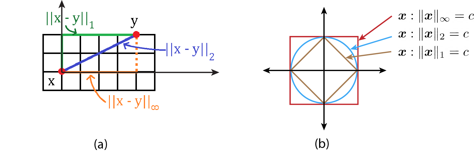
1. 1-norm: The 1-norm of $\vx$ is $\|\vx\|_1:=|x_1|+\dots+|x_n|$.
2. Sup-norm: The sup-norm of $\vx$ is the largest entry of $\vx$ in absolute value, i.e. $\|\vx\|_\infty = \max_{j}|x_j|$.
3. p-norm: For $p\geq 1$, the p-norm of $\vx$ is $\|\vx\|_p = \left(\sum_{j=1}^n|x_j|^p\right)^\tfrac{1}{p}$.

Linear functions

Linear function in a mapping between two Eucliean spaces that preserve the operations of addition and scalar multiplication. Specifially, a function $\func{f}:\R^n\rightarrow\R^m$ is linear if for all $\vx,\vy\in\R^n$ and $\alpha\in\R$, we have

$$\func{f}(\alpha\vx+\vy) = \alpha\func{f}(\vx)+\func{f}(\vy)$$

Here, $\func{f}$ takes a vector of dimension $n$ as its input and outputs a vector of dimension of $m$. If $m=1$, then we say the function $\func{f}$ is a real valued function.

$\prop$ A real valued function $\func{f}:\R^n\rightarrow \R$ is linear if and only if $\func{f} = \va^\intercal\vx$ for some $\va \in\R^n$.

$\proof$ We will first prove the forward direction, i.e. if $\func{f}:\R^n\rightarrow\R$ is a linear function then $\func{f}(\vx)=\va^\intercal\vx$. For $i\in\{1,\dots,n\}$, let $a_{i} = \func{f}(\ve_i)$. Then since $\vx = x_1\ve_1+\dots+x_n\ve_n$, we have

$$\begin{align*} \func{f}(\vx) &= \func{f}(x_1\ve_1+\dots+x_n\ve_n)\\ &=x_1\func{f}(\ve_1)+\dots+x_n\func{f}(\ve_n)\\ &= x_1\va_1+\dots+x_n\va_n\\ &= \va^\intercal\vx. \end{align*}$$

Second, we prove the reverse direction, i.e. if $\func{f}(\vx) = \va^\intercal\vx$ for some $\va \in \R^n$ then $\func{f}$ is a real valued linear function. Clearly, $\func{f}(x)$ is a real valued function. Let $\vx,\vy\in \R^n$ and $\alpha \in \R$. Consider

$$\begin{align*} \func{f}(\alpha\vx+\vy) &= \va^\intercal(\alpha\vx+\vy)\\ &=\va^\intercal(\alpha\vx)+\va^\intercal\vy\\ & = \alpha \va^\intercal\vx+\va^\intercal\vy\\ & = \alpha\func{f}(\vx)+\func{f}(\vy) \end{align*}$$

where the second inequality follows from linearity of inner product. q.e.d.