Linear Constraint¶

In this lecture, we consider optimization problem where the unknown variable satisfies a linear constraint. Let $f:\R^n → \R$ be a continuously differentiable real valued function and $\mA \in \R^{m\times n}$ be a matrix with $m\le n$ . The linearly-constrained optimization problem is

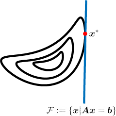
$\begin{equation}\label{linear_constraint} \minimize_{\vx\in\R^n} f(\vx) \text{ subject to } \mA\vx = \vb, \end{equation}$

where $\vb \in \R^m$ is a fixed vector. We assume that the matrix $\mA$ has full row rank and the minimum value is finite and attained. The figure below shows interaction between the objective function $f$ and the feasible set $\mathcal{F}$ . The feasible set is the set of point that satisfy the constraint.

Reduced unconstrained problem¶

In the case of linear constraints as in \eqref{linear_constraint}, we can reformulate the problem into an unconstrained problem. In order to write the unconstrained problem, we note that the feasible set $\mathcal{F} = \{\vx \in \R^n| \mA\vx=\vb\}$ can we equivalent expressed as the set $\{\bar{\vx} + \mZ \vp |\vp \in \R^{n-m}\}$ , where

$\bar{x}$ is any particular feasible solution , i.e. $\bar{\vx}$ satisfies $\mA\bar{\vx} = \vb$ , and
$\mZ$ is a basis for $\vnull(\mA)$ .

So, any $\vx$ that satisfies the linear constraint in \eqref{linear_constraint} can be expressed as $\bar{\vx}+\mZ\vp$ for some $\vp \in \R^{n-m}$ . This reduces the linear constrained problem \eqref{linear_constraint} to an unconstrained problem in $n-m$ variables:

$\begin{equation}\label{reduced_unconstrained} \minimize_{\vp\in\R^{n-m}} f(\bar{\vx} + \mZ\vp). \end{equation}$

The above unconstrained problem can be solved to get an optimal $\vp^*$ via any unconstrained method. The corresponding optimal solution to the constrained problem is then $\vx^* = \bar{\vx}+\mZ\vp^*$ .

Optimality Conditions¶

Define "reduced" objective function for any particular solution $\bar{\vx}$ and basis for null space $\mZ$ as $f_\vz(\vp): = f(\bar{\vx} + \mZ\vp)$ . THe gradient of $f_\vx$ at $\vp$ is

$\nabla f_\vz(\vp) = \mZ\trans\nabla f(\bar{\vx} + \mZ+\vp).$

The quantity $\nabla f_\vz$ is called the reduced gradient. Let $\vp^*$ be an arbitrary point and set $\vx^* = \bar{\vx}+\mZ\vp^*$ . Then $\vp^*$ is optimal only if

$\nabla f_\vz(\vp^*) = 0 ⇔ \mZ\trans\nabla f(\vx^*) = 0 \Leftrightarrow \nabla f(\vx^*) \in \vnull(\mZ\trans).$

By construction of $\mZ$ , we have $\vnull(\mZ) = \range(\mA)$ . Also, note that the fundamental subspaces in $\R^n$ associated with $\mA$ and $\mZ$ satisfy

$\begin{align*} & \range(\mA\trans)\oplus \vnull(\mA) = \R^n,\text{ and}\\ & \vnull(\mZ\trans)\oplus \range(\mZ) = \R^n. \end{align*}$

Thus, $\nabla f(\vx^*) \in \vnull(\mZ\trans)$ if and only if $\nabla f(\vx^*) \in \range(\mA\trans)$ . Further, $\nabla f(\vx^*) \in \range(\mA\trans)$ if and only if there exist a $\vy$ such that $\nabla f(\vx^*) = \mA\trans\vy$ . These relations lead to the following first-order necessary conditions.

Lemma (First order necessary condition) A point $\vx^*$ is a local minimizer of \eqref{linear_constraint} only if there exists an $m$ -vector $\vy$ such that

(Optimality) $\nabla f(\vx^*) = \mA\trans\vy = \sum_{i=1}^m \va_i y_i$ . Here, $\va_i$ is the $i$ th row of $\mA$ .
(Feasibility) $\mA\vx^* = \vb$ .

Note that the optimality statement in the above lemma can be equivalently expressed as $\mZ\trans\nabla f(\vx^*) = 0$ , which is further equivalent to $\nabla f(\vx^*)\trans\vp = 0$ for all $\vp \in\vnull(A)$ . The vector $y$ is sometimes referred to as "Lagrange multipliers".

Note that the Hessian of $f_\vz$ at $\vp$ is $\nabla^2 f_\vz(\vp) = \mZ\trans\nabla^2f(\bar{\vx}+\mZ\vp)\mZ$ . We now state the necessary second-order condition.

Lemma (Second-order necessary condition) A point $\vx^*$ is a local minimizer only if $\mA\vx^* = \vb$ and $\nabla^2f_\vz(\vx^*)⪰ 0$ . Equivalently, $\vx^*$ is a local minimizer only if $\mA\vx^* = \vb$ and $\mZ\trans\nabla^2f(\vx^*)\mZ \succeq 0$ .

We now state the sufficient second-order optimality condition.

Lemma (Second-order sufficient condition) A point $\vx^*$ is a local minimizer if it satisfies the following conditions:

(Feasibility) $\mA\vx^* = \vb$ ,
(Stationary) $\nabla f_\vz(\vx^*) = 0$ , and
(Positivity) $\nabla^2f_\vz(\vx^*) \succ 0$ .

Equivalently, $\vx^*$ is a local minimizer if it satisfies the following conditions:

(Feasibility) $\mA\vx^* = \vb$ ,
(Stationary) $\nabla f(\vx^*) = \mA\trans\vy$ for some $\vy$ , and
(Positivity) $\vp\trans\nabla^2f(\vx^*)\vp>0$ for all $\vp \in \vnull(A)\backslash \{\vzero\}$ .

Example¶

(Least norm solutions) Consider the following problem:

$\minimize_{\vx} \|\vx\|_2 \text{ subject to } \mA\vx=\vb.$

To find the least norm solution, we first state the corresponding first-order optimality condition. Without loss of generality, we may assume that the objective is $f(\vx) = \frac{1}{2}\|\vx\|_2^2$ . Since $\nabla f(\vx) = \vx$ , first-order optimality is

$\left. \begin{array}{c} &\vx = \mA\trans\vy \text{ for some } \vy\\ &\mA\vx = \vb \end{array} \right\} ⇔ \bmat-\mI & \mA\trans\\ \mA & \vzero\emat\bmat\vx\\ \vy\emat = \bmat\vzero\\ \vb\emat.$

So, if the constraint set $\mA\vx = \vb$ is $x_1 + x_2 + \dots + x_n = 1$ , then the first order optimality condition yields

$\bmat-\mI & \ve \trans\\ \ve\trans & 0\emat\bmat\vx\\ y\emat = \bmat 0\\ 1\emat \Rightarrow \left\{\begin{array}{c} &-vx +\ve y = 0\\ &\ve\trans\vx = 1 \end{array}\right\} \Rightarrow \ve\trans\ve\vy = 1 ⇒ y = \frac{1}{n}.$

Thus, the minimizer is $\vx = \frac{1}{n} \ve$ .

Algorithm¶

The reduced gradient method for solving linear constraint optimization problem is:

Algorithm (Reduced gradient method)

Given $\vx_0$ feasible and $\mZ$ a basis for $\vnull(\mA)$

For $k = 0, 1, 2, \dots$

Compute $\vg := \nabla f(\vx_k)$ .
Compute $\mH := \nabla^2f(\vx_k)$ .
Solve $\mZ\trans\mH\mZ\vp = -\mZ\trans\vg$ to get $\vp_k$ .
Linesearch on $f(\vx_k + \alpha \mZ\vp_k)$ .
$\vx_{k+1} = \vx_k + \alpha_k\mZ\vp_k$ .
Repeat until convergence.

The algorithm requires an initial feasible point and a basis for the null space of $\mA$ . An initial feasible point is easy to obtain (for example, the least squares solution). One approach to obtain a basis for the null space is by considering the QR decomposition of $\mA\trans$ . We will present an alternate way to construct the basis for the null space.

Permute the columns of $\mA$ so that the matrix $\mA$ can be represented as

$\mA = \bmat \mB & \mN\emat,$

where $\mB$ is non-singular. Such a matrix exists because $\mA$ is full rank. The matrix $\mB$ is called a basic matrix and $\mN$ is called the non-basic matrix. Then feasibility requires

$\mA\vx =\vb ⇔ \bmat\mB &\mN\emat\bmat\vx_B\\ \vx_N\emat \Leftrightarrow \mB\vx_B + \mN\vx_N = \vb.$

The variables $\vx_B$ and $\vx_N$ are called basic variable and non-basic variable respectively. Note that $\vx_B$ is uniquely determined by $\vx_N$ , i.e. $\vx_B = \mB^{-1}(b-\mN\vx_N)$ , and $\vx_N$ is free to move.

By construction, the matrix $\mZ = \bmat-\mB^{-1}\mN\\ \mI\emat$ is a basis for the null space of $\mA$ . This is because $\mA\mZ = \bmat\mB&\mN\emat\bmat-\mB^{-1}\mN \\ \mI\emat = 0$ .