Regularized least squares

In the least squares problem, we minimized 2-norm squared of the data misfit relative to a linear model. In contrast to the least squares formulation, many problem need to balance competing objectives. For example, consider the problem of finding $\vx_0 \in \R^n$ from noisy linear measurements $\vb = \mA\vx_0 + \vw_\vb$ and $\vg = \mF\vx_0-\vw_\vg$. Here $\vw_\vb$ and $\vw_\vg$ are noise vectors. In order to solve this problem, we need to find a $\vx$ that makes

1. $\func{f}_1(\vx) = \|\mA\vx - \vb\|_2^2$ small, and
2. $\func{f}_2(\vx) = \|\mB\vx - \vg\|_2^2$ small.

Generally, we can make $\func{f}_1(\vx)$ or $\func{f}_2(\vx)$ small, but not both. The figure below shows this relationship between $\func{f}_1(\vx)$ and $\func{f}_2(\vx)$.

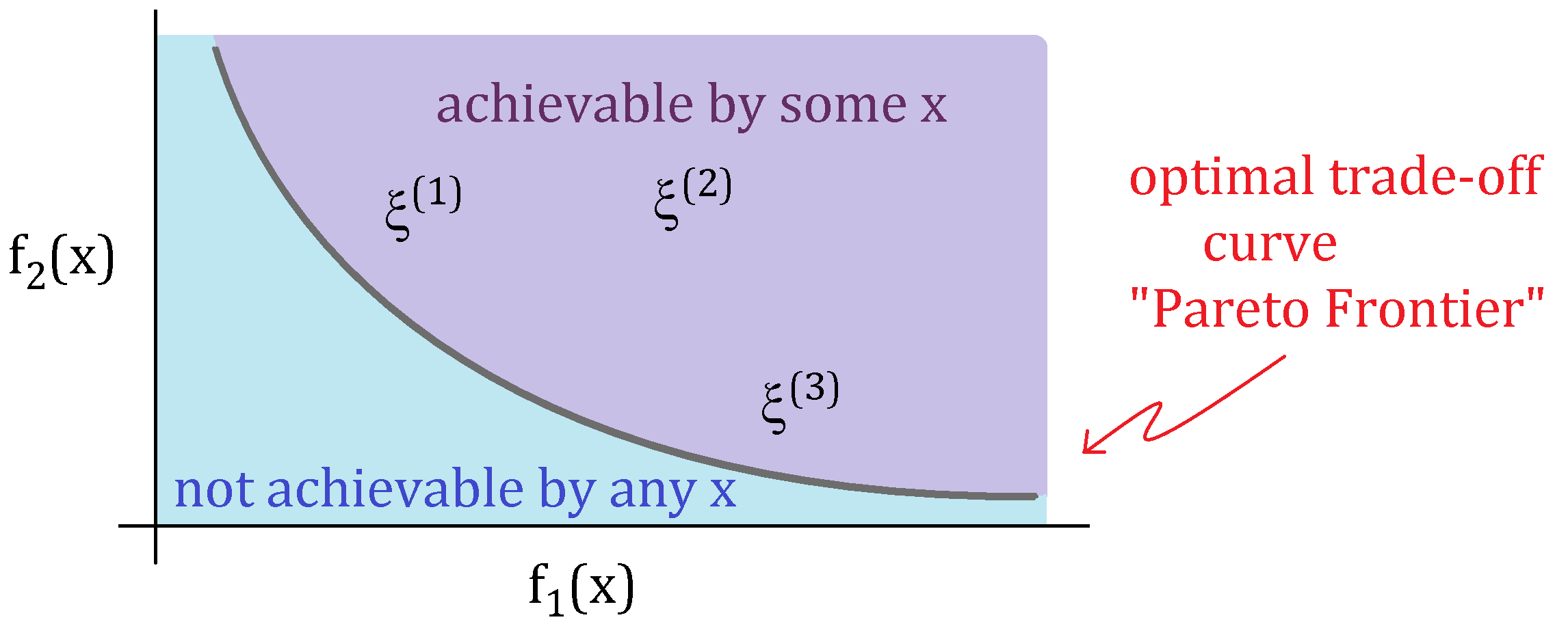
In the figure, the points in the boundary of two regions are called the Pareto optimal solutions. In order to find these optimal solutions, we minimize the following weighted sum objective:

$$\begin{equation}\label{Regularized_LS_weight} f_1(\vx)+\gamma f_2(\vx) = \|\mA\vx-\vg\|_2^2+γ\|\mF\vx-\vg\|_2^2. \end{equation}$$

The parameter $\gamma$ is non-negative and defines relative weight between the objectives. For example, in the case of $\gamma =1$, the optimal point that minimizes \eqref{Regularized_LS_weight} is the point $\vx$ on the optimal trade-off curve with $f_1(\vx) = f_2(\vx)$.

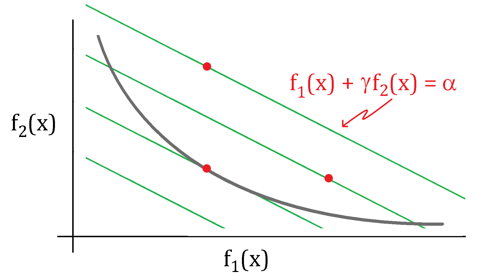
Note that for a fixed $\gamma$ and $\alpha \in \R$, the set

$$\ell(\gamma,\alpha) = \{(f_1(\vx),f_2(\vx)):f_1(\vx) +\gamma f_2(\vx) = \alpha, \vx \in \R^n\}$$

correspond to a line with slope of $-\gamma$. Another way to visualize the optimal solution is to find the line that is tangent to the optimal trade-off cuve, see figure below.

Example: Signal denoising

Suppose we observe noisy measurements of a signal:

$$\vb = \hat{\vx} + \vw,$$

where $\hat{\vx}\in\R^n$ is the signal and $\vw \in \R^n$ is noise. A simple apporach to find $\hat{\vx}$ is to solve:

$$\min_{\vx\in\R^n} \frac{1}{2}\|\vx-\vb\|_2^2.$$

This minimization program doesnot enforce any structure on $\vx$. However, if we have prior information that the signal is "smooth", then we might balance the least squares fit against the smoothness of the solution in the following way:

$$\begin{equation}\label{Regularized_LS_identity} \min_{\vx\in\R^n} \frac{1}{2}\|\vx-\vb\|_2^2 +\frac{\gamma}{2} \underbrace{\sum_{i=1}^{n-1}(x_i - x_{i+})^2}_{f_2(\vx)}. \end{equation}$$

Here, $f_2(x)$ promotes smoothness. We can alternatively write the above minimization program in matrix notation. Define the finite differencem matrix

$$\mD = \bmat 1 & -1 & 0 & \cdots & 0 & 0\\ 0 & 1 & -1 & 0 & \cdots & 0\\ & & \ddots & \ddots & & \\ 0 & \cdots & 0 & 1 & -1 & 0\\ 0 & 0 & \cdots & 0 & 1 & -1\emat \in \R^{{n-1}\times n}$$

So, we can rewrite $f_2(\vx) = \sum_{i=1}^{n-1}(x_i - x_{i+})^2 = \|\mD\vx\|_2^2$. This allows for a reformulation of the weighted leas squares objective into a familiar least squares objective:

$$\|\vx-\vb\|_2^2+\gamma\|\mD\vx\|_2^2 = \bigg\|\underbrace{\bmat\mI\\\sqrt{\gamma}\mD\emat}_{\hat{\mA}}\vx - \underbrace{\bmat\vb\\ \vzero\emat}_{\hat{\vb}}\bigg\|_2^2.$$

So the solution to the weighted least squares minimization program \eqref{Regularized_LS_identity} satisfies the normal equation $\hat{\mA}\trans\hat{\mA}\vx = \hat{\mA}\trans\hat{\vb}$, which simplifies to

$$(\mI + \gamma\mD\trans\mD)\vx = \vb.$$

Regularized least squares (aka Tikhonov)

We now generalize the result to noisy linear observations of a signal. In this case, the model is

$$\vb = \mA\vx + \vw,$$

where we added the measurement matrix $\mA \in \R^{m\times n}$. The corresponding wighted-sum least squares program is

$$\begin{equation} \min_{\vx\in\R^n} \frac{1}{2}\|\mA\vx-\vb\|_2^2 + \frac{\gamma}{2}\|\mD\vx\|_2^2, \end{equation}$$

where $\|\mD\vx\|_2^2$ is called the regularization penalty and $\gamma$ is called the regularization parameter. The objective function can be reformulated as an least squares objective

$$\|\mA\vx-\vb\|_2^2+\gamma\|\mD\vx\|_2^2 = \bigg\|\underbrace{\bmat\mA\\\sqrt{\gamma}\mD\emat}_{\hat{\mA}}\vx - \underbrace{\bmat\vb\\ \vzero\emat}_{\hat{\vb}}\bigg\|_2^2.$$

and the corresponding normal equations is

$$(\mA\trans\mA + \gamma\mD\trans\mD)\vx = \mA\trans\vb.$$